In this blog post I will look at how to optimize a battery schedule using a Mixed Integer Linear Programming (MILP) formulation of the problem. I use data from a recent data-driven competition, which investigated using batteries to minimize a site’s electricity bill. I used this in a paper recently (Projecting battery adoption in the prosumer era in Applied Energy) and this post documents the problem formulation. All the code and data is available in this repository containing a jupyter notebook which goes along with this post. This post is written to go along with the code in the repo. The repository also contains an alternative formulation (also used in the paper) as well as notebook which applies the formulation to all test data set of the data driven competition to generate a score.

Getting set up

First of all, one needs to get set up with pyomo and CPLEX, which are the modelling language and the solver we will use. I wrote myself a rough set of notes for what I did to get set up and running with CPLEX/pyomo in jupyter notebooks on a linux server, and they might help… but I also imagine you can find some better resources for this – here is a link to the actual pyomo documentation.

Scheduling a battery using pyomo and MILP

Secondly, we need some data about electricity prices and battery properties. Additionally, since the problem is a little bit boring with only a single set of prices and more often than not people are interested in batteries deployed at a specific consumer site, we will consider batteries located at consumer sites with demand and generation, where there is a buy price and a sell price for electricity. Conveniently, the data can then come from the competition!

Our aim is to use the battery to reduce or increase the site load at different times, in order to minimize the site electricity bill. Since there are buy prices and sell prices for electricity, there is a difference between reducing the load to zero (i.e. reducing the amount the site must buy) and reducing the load below zero (i.e. increasing the amount that the site is selling). Each site has a PV installation, so there is both demand and generation, but the price at each period only depends on the net load. The demand ($d(t)$), PV generation ($PV(t)$), buy price ($buyPrice(t)$) and sell price ($sellPrice(t)$) are timeseries with a fixed value at each time period.

To calculate the net load, we sum the demand, the generation and the battery action at each period, as shown.

$netLoad(t) = d(t)+PV(t)+ES(t)$ (1)

The price at each period is given either by the buy price, if the site is importing electricity, or the sell price, if the site is exporting electricity. This is summarised conditionally as follows:

IF $ Net(t) > 0, price(t)=buyPrice(t) $, ELSEIF $ Net(t) < 0, price(t)=sellPrice(t) $ (2)

We can see from the first equation that the unknown is the input/output of the battery, $ES(t)$ (if there is no battery then this term is equal to zero at all times)

The battery is then defined by its characteristics. We model a battery with the following parameters:

1. Maximum and Minimum states of charge, $SOC_{max}$ and $SOC_{min}$
2. Charging and discharging power limits (which could be different, but in the example we assume they are equal)
3. Charging and discharging efficiency ($\eta_{Char}$ and $\eta_{Dis}$, which again can be different, but we assume that they are equal and so the roundtrip efficiency is the product of the charging and discharging efficiency).

It must be noted here that this is a very simple battery model that does not take into account potentially important factors such as temperature, depth of discharge, applied current and voltage.

Now that we are done with the definitions we can go into the modelling procedure. As I mentioned earlier, we will use data from the recent data driven competition. The competition provided two datasets, a training set and a testing set. We will just use the testing set, since we are developing a data-independent model. In the competition, the demand was unknown and a forecast was given, and additionally the prices were only specified 1 day into the future. Hence, the training set was introduced so that competitors could learn specific features about each site and improve their algorithms.

Since we are interested in obtaining the optimum battery schedule, we will just take all the information we need from the testing dataset (in a folder called submit - you may need to sign up to get access - it is also all available in my repository). Therefore, for our chosen site (siteId=1) we will take values for the actual demand, actual PV generation and electricity prices for both buying and selling from the data provided (we won’t use the price, demand and generation forecasts at each period).

We will get the battery parameters from the metadata file from the competition repo:

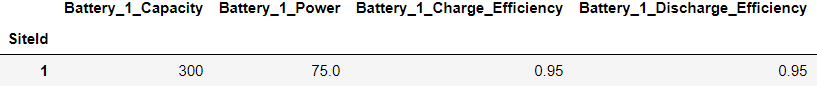
Fig. 1: The dataframe header showing battery properties

So we will initially model a battery with a capacity of 300 kWh, a charging power of 75 kW and a roundtrip efficiency of $\eta_{Char} \eta_{Dis} = (0.95)^2$.
Now let’s look at the data from site 1.

The data is in a csv file and it is easiest to access using pandas. It is split into different 10 day periods so we will just look at the first one.

Here is a plot of the demand and generation as well as the buy and sell prices for electricity.

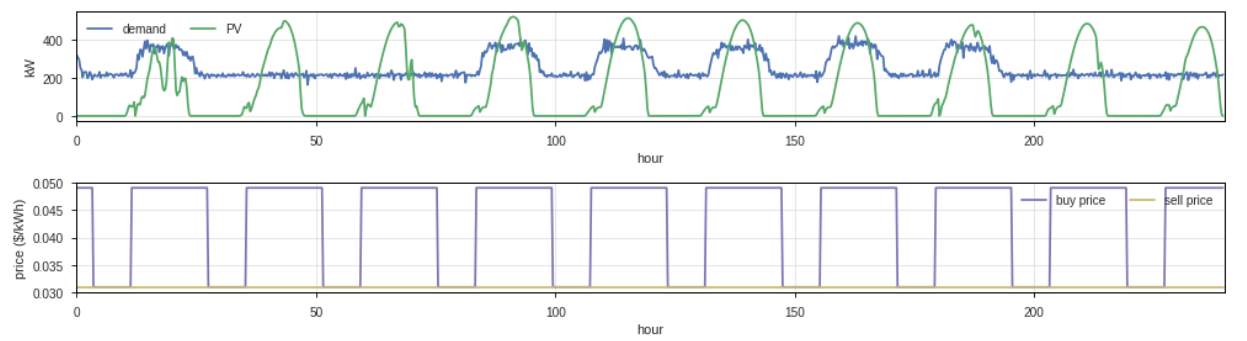
Fig. 2: Demand and generation from site 1 as well as the electricity prices

We can see that at certain times $PV(t)>demand(t)$ and therefore the site will be exporting electricity at the sell price. Looking the price profile, we can also see that the export price is always a constant level which is less than the highest buy price. Therefore, we get the intuition that the optimum battery operation is likely to store electricity that would be sold and use it to replace electricity that would have to be bought at expensive times.

To set up the optimisation problem, we first define the variables and an objective function, which corresponds to the total price of the consumer electricity. Pyomo requires us to set up the problem algebraically. What this means is that we define a set of variables, the objective function and constraints on the variables. The majority of the difficulty of setting the problem up in this way is writing down the variables, their relationships to each other and constraints such that the problem makes sense and does exactly what we intend.

First off, we need to initialize the model, for which we will use the concrete model framework in pyomo (concrete model means that we will define all the parameters at the time of the model definition, as opposed to an abstract model where we formulate the problem algebraically and parameter values are specified at a later stage). We also set up the model index which will be our times.

# now set up the pyomo model
m = en.ConcreteModel()
# we use rangeset to make a sequence of integers
# time is what we will use as the index
m.Time = en.RangeSet(0, len(net)-1)

Now let’s write down the objective function taking in mind the Equations 1 and 2 above:

$ObjFn = SUM [buyPrice(t)*posNetLoad(t) + sellPrice(t)*negNetLoad(t)]$ (3)

$posNetLoad$ is the net load at every period if the net load is greater than zero and $negNetLoad$ is minus the net load at every period if the net load is less than zero. $posNetLoad$ and $negNetLoad$ are the decision variables.

Let's also write down rules governing the state of charge of the battery. This consists of two components; the rule governing the minimum and maximum states of charge and the rule governing how much the state of charge changes at each period. The rule governing the max and min states of charge is a simple constraint, and can be included using bounds on the variable SOC. In pyomo we can do this when initializing the variable:

$ 0 \leq SOC(t) \leq batteryCapacity$ (4)

# variables (all indexed by time)
m.SOC = en.Var(m.Time, bounds=(0,batt.capacity), initialize=0)

Integer constraints

Here is where the “mixed integer” part of the formulation comes in. We specify constraints ensuring that the battery can only either charge or discharge at a particular period. To do this we specify Boolean variables for charging and discharging, $boolChar(t)$ and $boolDis(t)$. We then bound the problem using the bigM method. Therefore, we formulate the following constraints:

$posDeltaSOC(t) \leq M(1-boolDis(t)) $ (5)
$posDeltaSOC(t) \geq -M*boolChar(t) $ (6)
$negDeltaSOC(t) \geq -M*boolDis(t) $ (7)
$negDeltaSOC(t) \leq M(1-boolChar(t)) $ (8)

The first constraint means that if the battery is discharging, the charging must be less than or equal to zero and the second forces it equal to zero. If the battery is charging then the first constraint imposes an upper limit that is at least two orders of magnitude greater than any feasible value and the second constraint imposes a redundant lower limit.

If discharging, the third constraint gives a lower limit to the discharging (remember discharging is –ve) and the fourth gives a redundant upper bound. If charging, the third and fourth constraints force $negDeltaSOC$ equal to zero.

To ensure that the battery cannot simultaneously charge and discharge at the same time we constrain that $boolChar(t)+boolDis(t) = 1$.

Other constraints and variable relationships

We then define $posDeltaSOC$ and $negDeltaSOC$ in terms of energy coming from the grid to the battery and energy coming from the PV, at this point ensuring that the charging efficiency decreases the amount of energy that actually makes it into the battery with the opposite for the discharging energy.

$posEInGrid(t)+posEInPV(t) = posDeltaSOC(t)/ \eta_{Char}$ (9)

Similarly,

$negEOutLocal(t)+negEOutExport(t) = negDeltaSOC(t)*\eta_{Dis} $ (10)

For the charging and discharging power limits, we must also use constraints rather than bounds, since we have split charging into the component which comes from the PV and that which comes from the grid. Therefore we have:

$posEInGrid(t)+posEInPV(t) \leq ChargingLimit $ (11)
$negEOutLocal(t)+negEOutExport(t) \geq DischargingLimit $ (12)

Then, to make sure that energy available for charging from PV is always less than or equal to the excess PV and the energy used locally must be less than or equal to the demand that is not met by PV, we specify the following constraints:

$posEInPV(t) \leq \mbox{ Initial negative }netLoad(t) $ (13)
$negEOutLocal(t) \geq \mbox{ -Initial positive }netLoad(t) $ (14)

Finally, we then define the decision variables in terms of the other variables:

$posNetLoad(t) = \mbox{ Initial positive } netLoad(t)+posEInGrid(t)+negEOutLocal(t) $ (15)
$negNetLoad(t) = \mbox{ Initial negative } netLoad(t)+posEInPV(t)+negEOutExport(t) $ (16)

Optimisation

Now that the problem is defined we can run the optimisation. We need to specify what tool we will use for the optimisation, which in our case will be cplex. Therefore we set:

opt = SolverFactory("cplex", executable="**insert you path here**")

And finally we can run!

# time it for good measure
t = time.time()
results = opt.solve(m)
elapsed = time.time() - t

Outputs

To get the model outputs, we cycle through the variables that we defined in the model component objects, and I prefer assigning each to a numpy array. Therefore, we loop through the model variable objects and assign the variables we want to arrays.

# now let's read in the value for each of the variables
outputVars = np.zeros((9,len(sellPrice)))
j = 0 
for v in m.component_objects(Var, active=True):
    print v.getname()
    # print varobject.get_values()
    varobject = getattr(m, str(v))
    for index in varobject:
        outputVars[j,index] = varobject[index].value
    j+=1
    if j == 9:
        break

Finally, we can then compare the consumer’s electricity bill with and without the battery, and look at what the optimal battery schedule and the consumer’s net demand are! We can also calculate the consumer’s electricity cost with the battery and compare this to their cost without the battery.

# get the total cost
cost_without_batt = np.sum([(buyPrice[i]*
	posLoad[i]/1000 + sellPrice[i]*negLoad[i]/1000) 
	for i in range(len(buyPrice))])
cost_with_batt = np.sum([(buyPrice[i]*
	outputVars[7,i]/1000 + sellPrice[i]*
	outputVars[8,i]/1000) for i in 
	range(len(buyPrice))])

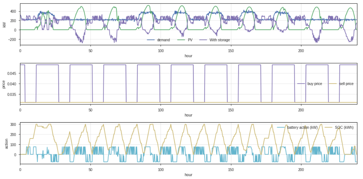
Fig. 3: The optimum battery operation for the site

Looking at the results we can see that the battery is doing the things we would expect – charging at the times when the price is low and discharging when the price is high. Finally, it is worth noting that in this example, there are a range of different optimum solutions – there are lots of different time options when the battery could charge and discharge at the same price (and the cost to the battery of PV-that-would-otherwise-be-exported is the same as the grid import price).

Concluding notes

The nice thing about using this setup is you can just keep adding more and more constraints and different forms of the cost function. For example, one could stipulate that a portion of the consumer’s electricity bill was related to their peak power usage. This allows one to model more and more complex electricity bill scenarios. However, as the problem gets more complicated, you need to be careful about what methods you are using to solve the problem, which is beyond the scope of this post (see the CPLEX manual for details regarding the type of problems it can solve). Additionally, as the number of constraints increases the computational time required will increase.

I wrote this post primarily because when I was first looking into MILP formulations, I didn't find many easily accessible examples of code that had been used for this type of exercise in academic papers. Therefore, I wanted to document my process.

Finally, thanks to my colleague, Alejandro Pena Bello at the University of Geneva first suggested that I try pyomo for MILP formulations in python and shared some code with me, which was super helpful. Additionally, I found these notes from MIT opencourseware useful when trying to understand how to set the problem up. The tutorials were also helpful.